Gradient descent with a visible loss calculation

Gradient descent updates parameters in the direction opposite the loss gradient. The learning rate controls the step size. A correct gradient does not guarantee decreasing loss when the step is too large.

Use a one-parameter example to make every quantity visible before applying the method inside a larger model. The original fixture below is noiseless training data, so convergence does not demonstrate predictive generalization.

Define the prediction and loss

The inputs are x = 1, 2, 3 and targets y = 2, 4, 6. Predict theta × x with no intercept. The mean squared error is the average of (theta × x - y)².

Because y is exactly 2x, the loss simplifies to (14/3) × (theta - 2)². Its derivative is (28/3) × (theta - 2). At theta zero, the loss is 56/3, about 18.667, and the gradient is -56/3.

With learning rate 0.05, the first update is 0 - 0.05 × (-56/3), giving theta approximately 0.9333. The next loss is about 5.3096, lower than the starting loss.

Check the derivative and updates

import numpy as np
from math_core import loss,gradient,descend

assert np.isclose(loss(0),56/3)
assert np.isclose(gradient(0),-56/3)
h = 1e-6
numerical = (loss(1.2+h)-loss(1.2-h))/(2*h)
assert np.isclose(numerical,gradient(1.2),rtol=1e-8)
good = descend(rate=.05,steps=30)
bad = descend(rate=.3,steps=6)
assert np.isclose(good[1]['theta'],14/15)
assert all(b['loss']<a['loss'] for a,b in zip(good,good[1:]))
assert abs(good[-1]['theta']-2)<1e-7
assert all(b['loss']>a['loss'] for a,b in zip(bad,bad[1:]))
print({'first_update':good[1],'small_rate_final':good[-1],
       'large_rate_step_6':bad[-1]})

The mathematics lab includes the CSV and functions. The finite-difference calculation independently checks the analytic gradient near theta 1.2 using a small symmetric perturbation.

See why the large step fails

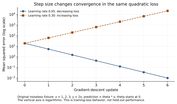
Open the full-size SVG for zooming. The figure plots the first six updates from the same checked functions.

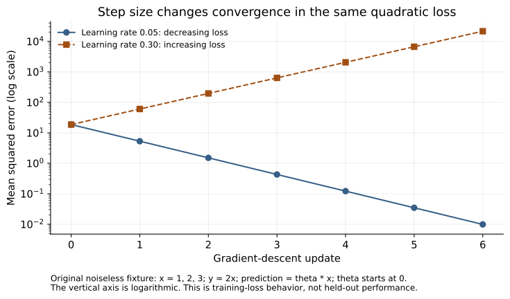
For this quadratic, the parameter error after an update is multiplied by 1 - learning_rate × 28/3. At 0.05, that factor is about 0.5333, so the error shrinks. At 0.30, it is -1.8, so the parameter crosses the optimum and moves farther away on each step.

The convergence condition for this particular fixed-step quadratic is an absolute multiplier below one: the learning rate must lie between zero and 3/14. This is a derived property of the example, not a universal recommended learning rate for machine learning.

Interpret the curve correctly

The vertical axis is logarithmic because the two trajectories span very different loss magnitudes. Equal vertical distances represent multiplicative changes, not equal absolute changes.

At six updates, the small-rate loss is about 0.00989, while the large-rate loss is about 21,594.19. At thirty small-rate updates, theta is within about 1.3e-8 of two in the recorded run.

These are training-loss results on three points generated exactly from the fitted model form. They do not establish how a model would behave with noise, an intercept, different feature scales or unseen data.

Use the example as a debugging method

When a larger model's loss behaves unexpectedly, inspect the loss definition, gradient scale, learning rate and input scaling. Test a small case with a known result. A sign error in the update and an excessive step can both increase loss, but they require different repairs.

Finite differences are useful for checking a small derivative implementation, although the perturbation size and floating-point precision affect the comparison. They are not a replacement for efficient gradient computation in a large training system.

Exercise: try a learning rate of 0.15. Predict whether the parameter approaches the optimum from one side or alternates around it, then inspect the loss and parameter history separately.

NeuraPath's Data Science course connects optimization mathematics with model training. A visible loss calculation helps you diagnose learning behavior rather than treating the optimizer as an unexplained command.

Continue learning

This article is part of the Mathematics and statistical foundations sequence. Use the neighbouring tasks when you need the prerequisite or the next application.

• Review the prerequisite or neighbouring task in Eigenvectors and PCA through a two-feature dataset.
• Continue with Partial derivatives: understand a model's local sensitivity.