Eigenvectors and PCA through a two-feature dataset

In covariance-based principal component analysis, eigenvectors identify orthogonal directions and eigenvalues describe the sample variance along those directions. Keeping the direction with the largest eigenvalue gives a one-component representation that preserves the most variance under this linear projection criterion.

High retained variance is not the same as high predictive usefulness. PCA does not use a target label in this example, so a low-variance direction could still matter to a later supervised task.

Center four inspectable points

The original points are (1, 2), (2, 1), (3, 4) and (4, 3). Both feature means are 2.5. Subtract those means before calculating the sample covariance with denominator n - 1.

The covariance matrix has diagonal entries 5/3 and off-diagonal entries 1. Its eigenvalues are 8/3 and 2/3, so the first component accounts for 80% of the total sample variance.

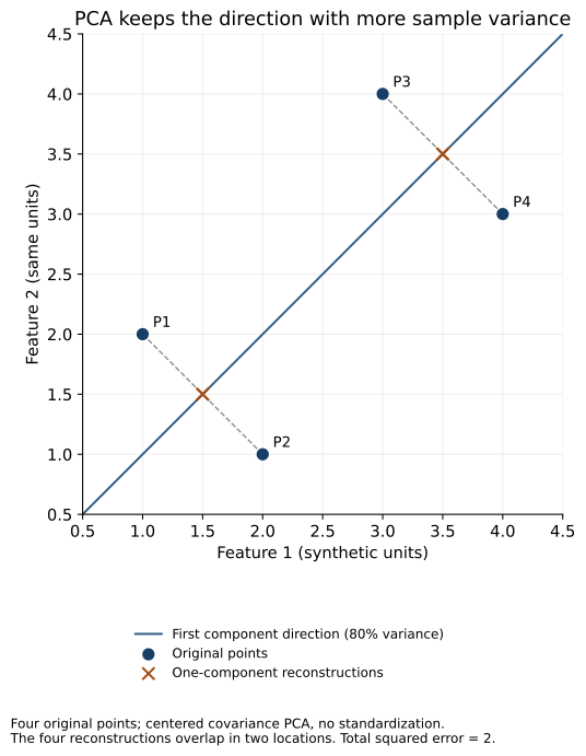
Open the full-size SVG for zooming. The lab includes the source CSV and renderer.

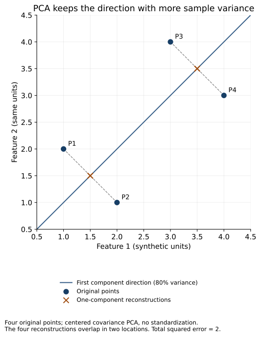
Verify the eigen relationship and reconstruction

import numpy as np
from sklearn.decomposition import PCA
from math_core import pca_reference,pca_data

r = pca_reference()
assert np.allclose(r['mean'],[2.5,2.5])
assert np.allclose(r['covariance'],[[5/3,1],[1,5/3]])
assert np.allclose(r['eigenvalues'],[8/3,2/3])
assert np.allclose(r['explained_ratio'],[.8,.2])
v = r['components_columns']
assert np.allclose(r['covariance']@v,v*r['eigenvalues'])
assert np.allclose(v.T@v,np.eye(2))
model = PCA(n_components=1,svd_solver='full').fit(pca_data())
reconstructed = model.inverse_transform(model.transform(pca_data()))
assert np.allclose(reconstructed,r['one_component_reconstruction'])
assert np.isclose(np.square(pca_data()-reconstructed).sum(),2)
print({'eigenvalues':r['eigenvalues'].tolist(),
       'retained_variance_fraction':float(model.explained_variance_ratio_[0]),
       'one_component_squared_reconstruction_error':2})

NumPy's symmetric eigenvalue routine supplies the eigen analysis. The independently fitted scikit-learn PCA uses the full SVD solver here and agrees on the reconstructed points. Local versions are NumPy 2.4.4 and scikit-learn 1.9.0.

Interpret the eigenvector sign correctly

An eigenvector and its negative describe the same axis. Software may return either sign. The corresponding component scores change sign too, leaving reconstruction unchanged.

The lab canonicalizes signs for readable output, but the verification compares the eigen relationship and reconstruction rather than treating one sign as the only correct answer. A sign difference between implementations is not automatically a model disagreement.

Understand what one component discards

The first direction follows the diagonal. P1 and P2 both reconstruct at (1.5, 1.5), while P3 and P4 reconstruct at (3.5, 3.5). Four reconstructed records therefore overlap at two visible locations.

The total squared reconstruction error is two. That is the sum of squared residuals over all four points and both features, not an 80% classification score or a claim of predictive accuracy.

The discarded direction accounts for the remaining 20% of sample variance. Whether discarding it is acceptable depends on the purpose of the representation.

Decide how scaling should work

This example gives both features comparable synthetic units and centers them without standardizing. PCA's result depends on feature scale. A feature measured in a larger numerical unit can dominate covariance even when that dominance is not useful for the task.

If you standardize, fit the transformation on the appropriate training data and preserve it for later observations. Do not fit PCA or scaling on a final test set and then describe the downstream evaluation as untouched.

Exercise: multiply the second feature by 100 and rerun the covariance PCA. Explain why the dominant direction changes and whether standardization would be a defensible choice for the intended feature meaning.

NeuraPath's Data Science course connects linear algebra with dimensionality reduction and model evaluation. A small PCA derivation helps you understand what the transformation preserves, what it discards and what its variance ratio cannot prove.

Continue learning

This article is part of the Mathematics and statistical foundations sequence. Use the neighbouring tasks when you need the prerequisite or the next application.

• Review the prerequisite or neighbouring task in Matrix multiplication: track shapes before calculating.
• Continue with Gradient descent with a visible loss calculation.