Standard deviation versus standard error with a simulation

Standard deviation describes variation among observations. The standard error of a mean describes variation in the estimated mean across repeated samples under a specified sampling model. They have the same units but answer different questions.

For independent, identically distributed observations with finite variance, the estimated standard error of the mean is the sample standard deviation divided by the square root of sample size. Dependence or a complex sampling design can invalidate that simple calculation.

Simulate repeated samples from a known process

The analyst statistics lab draws 5,000 independent samples, each containing 25 observations from a normal distribution with mean 100 and standard deviation 20.

import numpy as np
from scipy import stats

rng = np.random.default_rng(20260920)
samples = rng.normal(loc=100, scale=20, size=(5000, 25))
sample_sds = samples.std(axis=1, ddof=1)
sample_means = samples.mean(axis=1)
estimated_ses = stats.sem(samples, axis=1, ddof=1)
assert np.allclose(estimated_ses, sample_sds / np.sqrt(25))
average_sd = float(sample_sds.mean())
empirical_se = float(sample_means.std(ddof=1))
assert 19 < average_sd < 21
assert 3.8 < empirical_se < 4.2
print({'average_sample_sd': average_sd, 'sd_of_sample_means': empirical_se,
       'theoretical_se': 20 / np.sqrt(25)})

In the recorded environment, the average sample SD is approximately 19.843 and the standard deviation of sample means is approximately 3.962. The theoretical standard error under this model is 4.

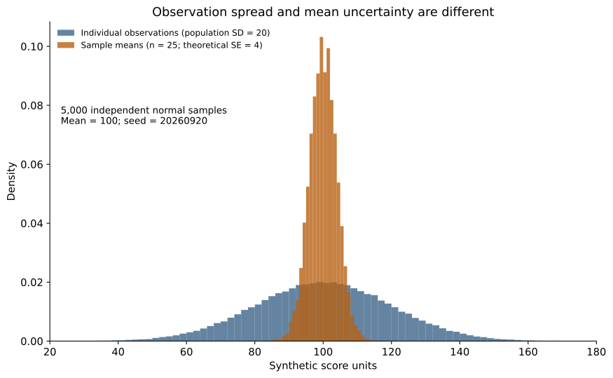
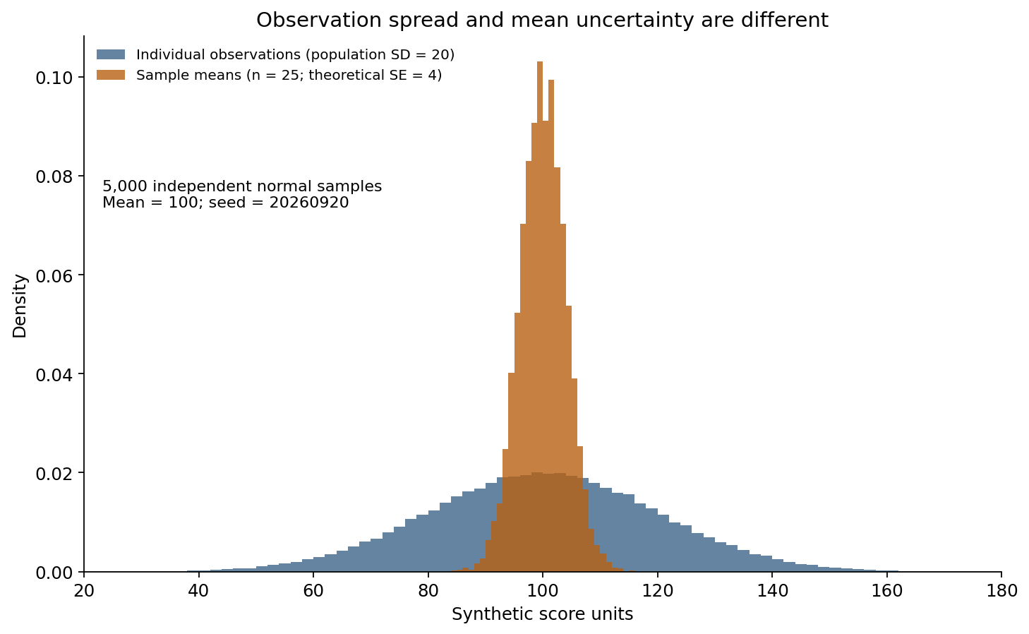
The figure uses the same seeded simulation. Both distributions use a density scale; the narrower orange distribution represents sample means, not less-variable individual observations. Download the PNG version or regenerate both formats with the lab's render_figures.py.

The SciPy sem reference documents the calculation and degrees-of-freedom setting. The simulated process and seed are stated explicitly so the numerical demonstration can be reproduced.

Explain why sample size changes one quantity

Increasing the number of independent observations improves precision in estimating the same population mean. It does not make individual observations less variable. The underlying process still has standard deviation 20.

Under this model, moving from n=25 to n=100 changes the theoretical standard error from 4 to 2. It does not change the population SD from 20 to 10.

That distinction matters when a chart uses error bars. SD bars show observed spread; SE bars show estimated precision of a mean. Label the bar type and do not expect the audience to infer it from the visual.

Do not count dependent rows as independent evidence

Twenty-five purchases from one customer may share preferences and circumstances. Twenty-five daily readings from one device may be autocorrelated. Treating those rows as twenty-five independent units can understate uncertainty.

Identify the sampling or randomization unit before applying the formula. Clustered data may require aggregation or a method that accounts for the dependence structure. Merely having a large row count is not enough.

Keep the estimand clear

The standard error discussed here belongs to the sample mean. A median, conversion rate or regression coefficient has a different uncertainty calculation. Do not divide an arbitrary metric's standard deviation by square root n and assume the result is its standard error.

Bootstrap or model-based methods can estimate uncertainty for other statistics, but they also require assumptions about how the data were generated and sampled.

Separate uncertainty from bias

A small standard error does not establish that the sample represents the target population. A biased collection process can estimate the wrong population mean very precisely.

The simulation is deliberately favorable: independent normal draws from the stated target distribution. Its numerical agreement demonstrates the formula under those conditions, not a guarantee for every operational dataset.

Exercise: repeat the simulation with n=100 and compare the spread of sample means with the spread of individual observations. Then create perfectly repeated copies of each observation and explain why the nominal row count should not be treated as new independent information.

NeuraPath's Data Analytics with Generative AI course connects statistical formulas with their data-design assumptions. A useful uncertainty statement says what varies, what is estimated and which units provide independent evidence.

Continue learning

This article is part of the Statistics for analytical decisions sequence. Use the neighbouring tasks when you need the prerequisite or the next application.

• Review the prerequisite or neighbouring task in Mean versus median in a skewed order-value report.
• Continue with Confidence intervals: explain uncertainty without promising certainty.