Law of large numbers versus central limit theorem
In this article (6 sections)
The law of large numbers concerns the sample mean becoming close to the population mean under suitable assumptions. The central limit theorem concerns the limiting distribution of the mean's appropriately standardized error. They describe related but different aspects of averaging.
Neither theorem says that every additional observation moves a particular running mean closer to the truth, or that collecting more biased measurements repairs the measurement process.
Compare the questions each theorem answers
In a familiar independent, identically distributed setting with a finite mean, the law of large numbers says the sample mean concentrates around that mean. In the classical finite-variance CLT setting, the standardized error approaches a normal distribution.
The MIT probability reading develops these distinctions. This article uses original exponential simulations rather than reproducing its examples.
| Question | Relevant idea |
|---|---|
| Does the mean concentrate near the population value? | Law of large numbers |
| What is the approximate shape of standardized mean error? | Central limit theorem |
| Is the measurement or sample biased? | Requires a separate data-design assessment |
| Will the next observation improve this exact running estimate? | Not guaranteed by either theorem |
See a running mean that moves both ways
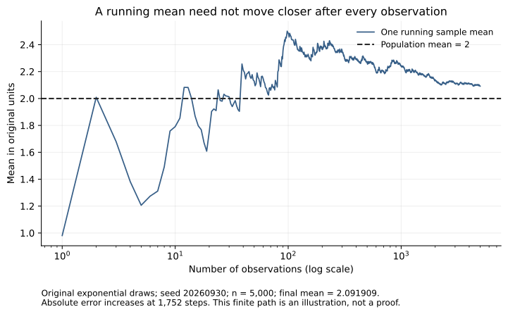
Open the full-size SVG for zooming. This is one seeded path, not a proof or a collection of independent estimates at every plotted point.
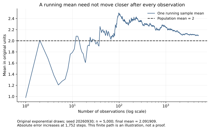
The final mean is approximately 2.0919 after 5,000 observations. Its absolute distance from two increases at 1,752 steps. Those increases do not contradict convergence: a sequence can converge without improving monotonically at every step.
Compare repeated-sample concentration
import numpy as np
from sampling_limits import summarize,running_path

r = summarize()
rows = r['independent_repeated_samples']
draws,path = running_path()
assert len(draws)==len(path)==5000
assert np.isclose(path[-1],draws.mean())
assert np.sum(np.diff(np.abs(path-2))>0)==1752
assert np.isclose(path[-1],2.0919085961489525)
assert rows[0]['fraction_mean_within_02_of_truth']==.07615
assert rows[-1]['fraction_mean_within_02_of_truth']==.67745
assert r['perfect_dependence_n100_mean_sd']>8*rows[-1]['sd_of_means_ddof1']
print({'within_0_2_of_truth_n1':.07615,'within_0_2_of_truth_n100':.67745,
       'running_final_mean':float(path[-1]),
       'perfect_dependence_mean_sd':r['perfect_dependence_n100_mean_sd']})
Across 20,000 repeated samples, about 7.615% of n=1 means fall within 0.2 of the population mean, compared with 67.745% of n=100 means in the recorded runs. That illustrates increasing concentration for the chosen tolerance and distribution.
The lab preserves the seeds, assumptions and exact outputs. The percentages are simulation observations, not universal probabilities for arbitrary data.
Explain why standardization matters
As the unstandardized mean concentrates, its spread shrinks. The CLT rescales the error by the square root of sample size and the population standard deviation to study a nondegenerate limiting shape.
For the exponential population with mean and SD both two, the theoretical standard error is 2 / sqrt(n) under independence. At n=100 it is 0.2. The standardized SD stays near one in the simulation even while the original-scale SD decreases.
This is why “the mean approaches the truth” and “the standardized error approaches normality” are compatible statements rather than competing explanations.
Do not count repeated copies as new evidence
The lab's dependence counterexample repeats one draw within each hypothetical sample of one hundred entries. The average is still that original draw. Its observed spread is about 1.981, not the roughly 0.2 spread of independent n=100 means.
Real data may have less extreme dependence, but the lesson remains: row count alone does not establish independent information. Repeated customers, clustered observations and time dependence need an appropriate analysis design.
Exercise: explain why averaging more readings from a systematically miscalibrated instrument may estimate the wrong quantity precisely. Identify which problem the LLN addresses and which requires a measurement correction.
NeuraPath's Data Science course connects mathematical assumptions with practical evaluation. Distinguishing concentration, distributional approximation and data quality helps you reason about what a larger dataset actually improves.
Continue learning
This article is part of the Mathematics and statistical foundations sequence. Use the neighbouring tasks when you need the prerequisite or the next application.
- Review the prerequisite or neighbouring task in Central limit theorem: simulate what actually converges.
- Continue with Likelihood versus probability in a fitted model.
Pankit Kumar has 10 years in Data Science & AI, building and shipping production systems in regulated pharma and clinical environments. He is a freelance trainer at Boston Institute of Analytics, AnalytixLabs and Scaler, and has taught this material to thousands of working professionals.
This article is part of our Data Science programme — 6 months. From data foundations to machine learning, deep learning and deployment.
Explore Data Science